Correlation Networks in R

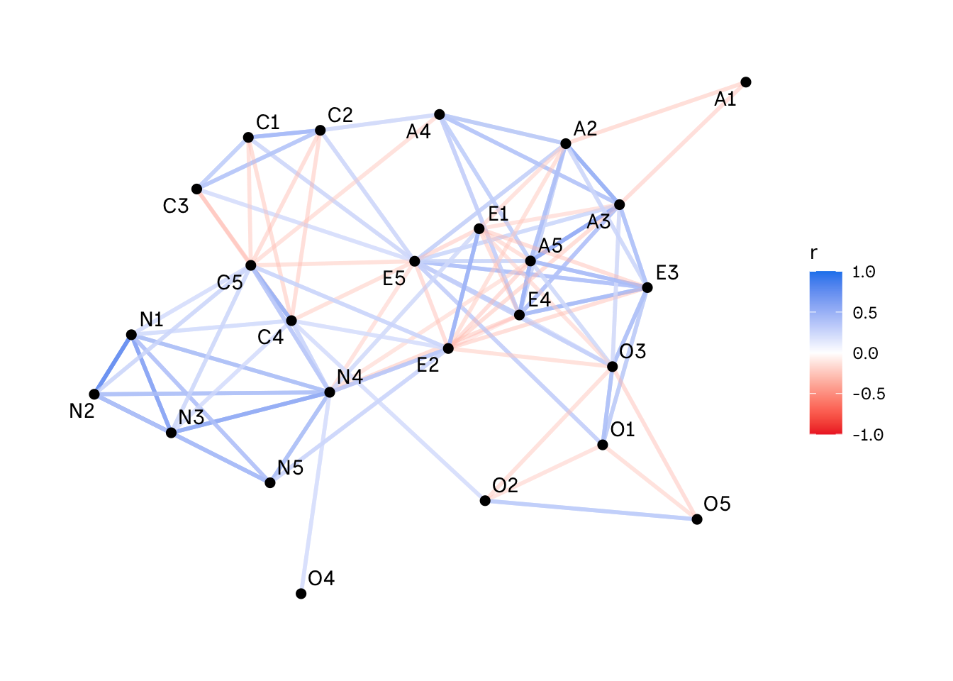
Plotting correlations as networks can give you a good first impression of the interconnectivity of your variables. This is a quick tutorial on how to create correlation networks in R.

To create a correlation network, we will use the BFI personality data from the {psych} package. First we will import all the necessary packages and set the font for our plot. We can import these from our system using extrafont. In the next step we will do a quick clean up of our data to include only the columns we want to visualise.

library(tidyverse)
library(ggraph)
library(igraph)
library(corrr)
library(extrafont) # font_import() to import your system fonts

font = "Inclusive Sans"

df <- psych::bfi %>%
  tibble() %>%
  select(-c(age, education, gender))

The correlate() function from the {corrr} package allows us to define a specific correlation. However, we will use the Pearson correlation as the default setting. Next, we will switch to a long format using stretch() and only keep correlations higher than .2 or lower than -.2. This is something to play around with. Depending on how many variables you have in your data, your plot could get really messy if you include all the possible relationships between your variables.

graph_data <- df %>% 
    corrr::correlate() %>% 
   corrr::stretch() %>% 
    filter(abs(r) > .2)

The last step is to build our visualisation. The font variable is the one we set above. In comparison to out of the box tools, this approach with {ggraph} and {igraph} allows us to adjust all the settings you are interested in, such as the size or colour of the nodes. We might also choose a different color scaling, for example if we only include postive correllations. In this specific example, I changed the background color to transparent.

graph_data %>%
    graph_from_data_frame(directed = FALSE) %>%
   ggraph(layout = "kk") +
    geom_edge_link(aes(color = r, alpha = r), edge_width = 1) +
    guides(edge_alpha = "none") +
    scale_edge_colour_gradientn(limits = c(-1, 1), colors = c("firebrick2", "white", "dodgerblue2")) +
    geom_node_point(color = "black", size = 2) +
    geom_node_text(aes(label = name), family = font, repel = TRUE) +
    theme_graph(base_family = font, title_size = 10) +
    theme(
      plot.background = element_rect(fill = "transparent", colour = NA),
        text = element_text(family = font),
        legend.title = element_text(family = font),
        legend.text = element_text(family = font)
    )