Introduction to partial residual plots

Partial residual plots can give you valuble information about your model and relationships in the data like interactions and nonlinear trends. In this post we look at use cases and different ways PRP can be created in ggplot.

What we missed

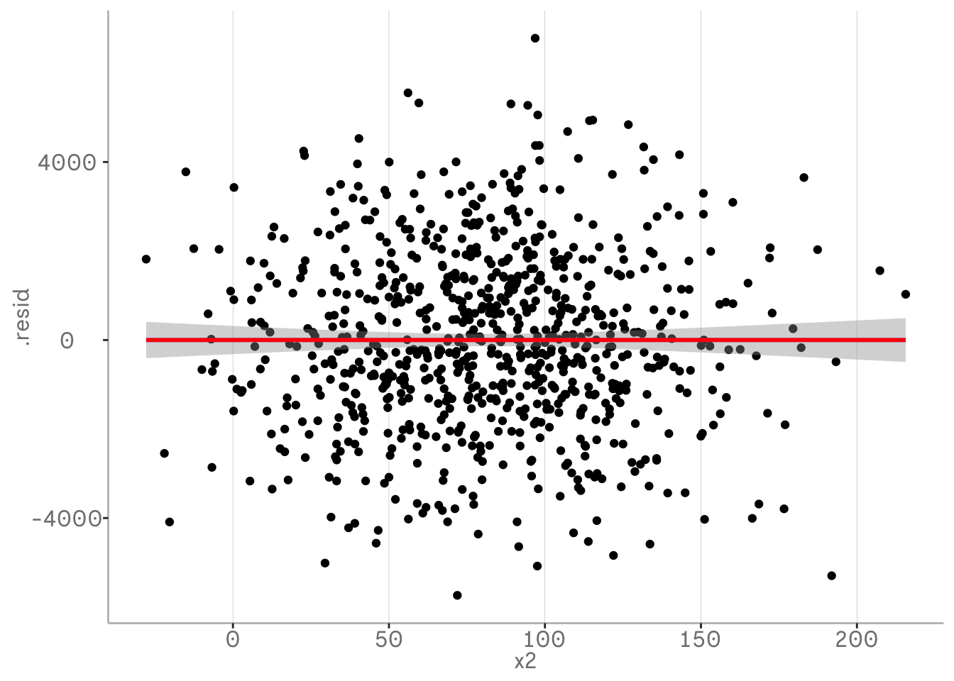
In a PRP, we plot the residuals, or error, of our regression model against one or more independent variables. This allows us to do a number of things - starting with the first: detect non-randomness in the residuals. Why is non-randomness important? When we run a regression, we assume that we have some error in the form of jitter around our predictions, which does not include any residual trend. This error is caused by all the things we do not know about our independent variable and cannot model. The theory assumes that if we had all the variables in the universe with a causal relationship to our independent variable, we could make predictions without error. However, this is fictional and error is part of our complex reality, which we can only approximate using such a naive linear representation of the world. It is only a problem when our error is not random, because then there is still some sort of trend or pattern in the data that we could have modelled with our variables. In practice, this can happen if there is some sort of non-linear trend in our data or interactions of variables that we need to include in our model.

In the following example we will first visualise the residuals from our regression using broom and ggplot by plotting them against one of our independent variables used in the model.

By using geom_smooth regression lines we can see the remaining trends in our residuals. The blue regression line is our tool for spotting these. Note that we want the intercept and slope to be approximately zero - this means there is no trend left. The red line represents the predictions of our model.

In the following plot you can not see the blue line, because they are exactly the same slope, which means that we have not detected any residual trends that our model has not picked up. At least for the variable x2.

m0 <- lm(y0 ~ x1 + x2 + x3)

m0 %>%
  broom::augment() %>% 
  ggplot(aes(x = x2, y = .resid))+
  geom_point()+
  geom_smooth(method = "lm")+
  geom_smooth(aes(x = x2, y = 0), method = "lm", color = "red")

In the second plot our blue regression lines indicate that there is still some pattern left in our variable x2 that is not included in our model. This is caused by a quadatric relationship that still remains in our residualds. This is a sign that we should adjust our model.

m1 <- lm(y_ac ~ x1 + x2 + x3)

m1 %>%
  broom::augment() %>% 
  ggplot(aes(x = x2, y = .resid))+
  xlim(c(50,190))+
  geom_point()+
  geom_smooth(method = "lm")+
  geom_smooth(aes(x = x2, y = 0), method = "lm", color = "red")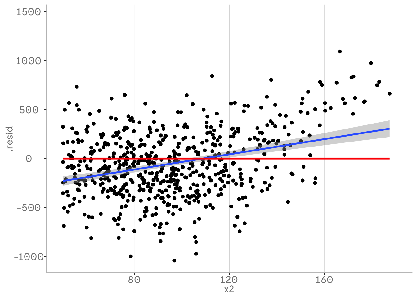

Spotting Interactions

In the plots above we have only looked at one variable in our model. However, we have several variables in our model and we may be interested in looking at them all. One way to do this is to pivot the data into a long format and plot them on a grid. In the following plot we can see that the residuals for x1 and x3 do not contain any unmodelled information, while the residuals for x2 do.

m1 <- lm(y_ac ~ x1 + x2 + x3)

m1 %>%
  broom::augment() %>% 
  pivot_longer(c(x1, x2, x3)) %>%
  ggplot(aes(x = value, y = .resid))+
  xlim(c(50,190))+
  geom_point()+
  geom_smooth(method = "lm")+
  geom_smooth(aes(x = value, y = 0), method = "lm", color = "red")+
  facet_grid(vars(name))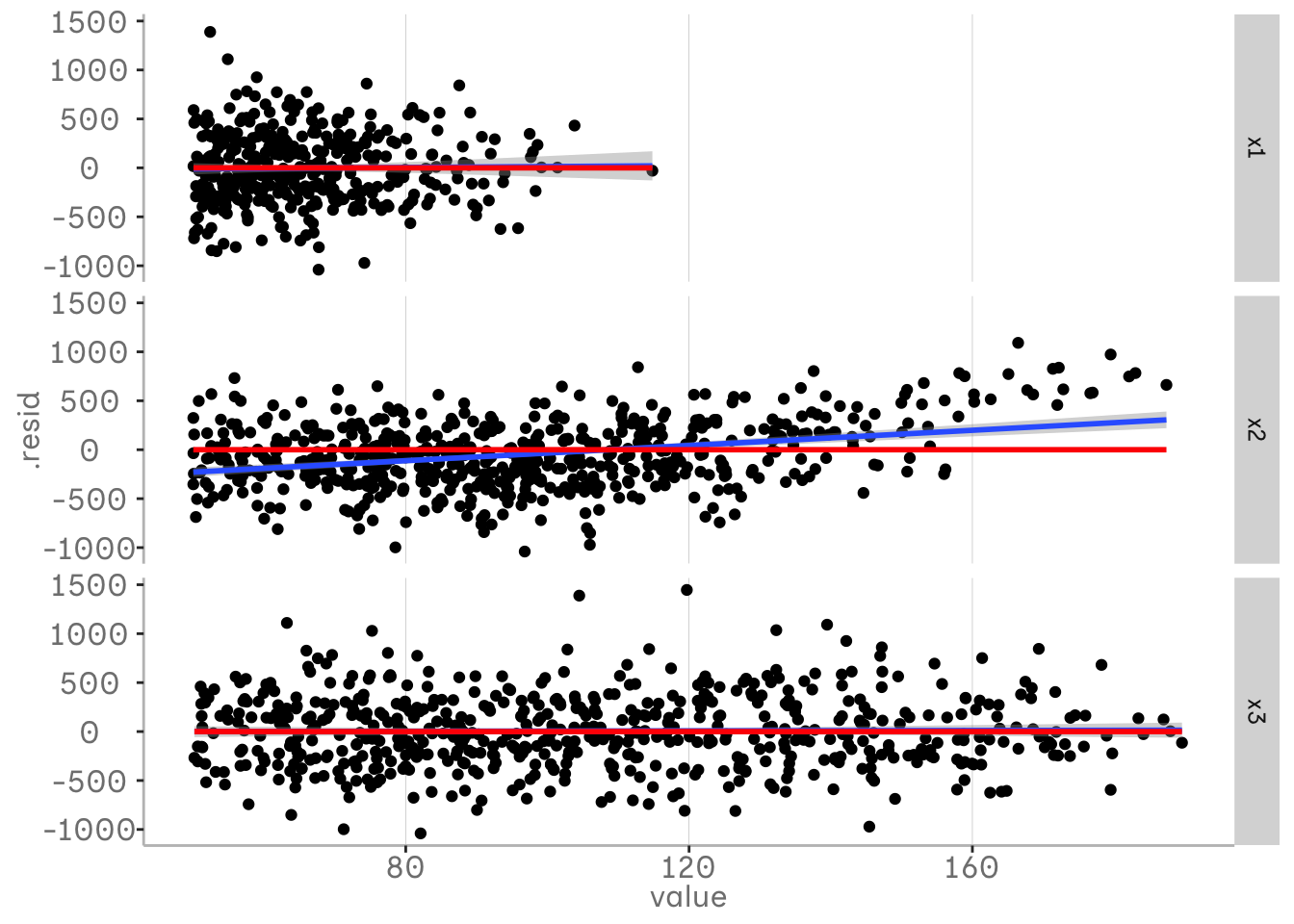

However, in this case we have only plotted our predictor variables against the residuals of our model and thus against our response variable. To see how our predictor variables are related to each other, we might want to plot them against each other as well. One way to do this is to plot them binned into quantiles in our grid. We can do this using the function dvmisc::quant_groups() and sort the values of x3 into 3 bins based on our quantiles.

This allows us to see interactions between our variables that are not in our model. In this plot you can see that the relationship between x1 and y changes at different quantiles of x3. At lower values of x3 there is a negative relationship between x1 and x3, while at higher values the relationship becomes more positive. We can see that our model does not currently account for this interaction.

m1 <- lm(y1 ~ x1 + x2 + x3)

m1 %>%
  broom::augment() %>% 
  mutate(x3 = dvmisc::quant_groups(x3, 3)) %>%
  pivot_longer(c(x1,x2)) %>%
  ggplot(aes(x = value, y = .resid))+
  xlim(c(50,190))+
  geom_point()+
  geom_smooth(method = "lm")+
  geom_smooth(aes(x = value, y = 0), method = "lm", color = "red")+
  facet_grid(vars(name), vars(x3))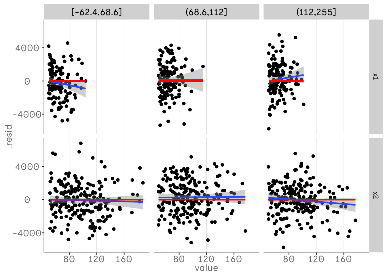

This method can also be used to detect three-way interactions. If we have already included a two-way interaction and still see a change in the relationship of one variable, there may be an additional interaction. In the following example, we have plotted x1 in our bins, so we can see how x2 and x3 vary for different quantiles of x1. We can see that there is no real trend left in the residuals when looking at x2 - we have already included the interaction for x2 and x1. For x3 we can see that there is some pattern left and this trend in the residuals varies over x1.

m3 <- lm(y1 ~ x1 * x2 + x3)

m3 %>%
  broom::augment() %>%
  mutate(x1 = dvmisc::quant_groups(x1, 3)) %>%
  pivot_longer(c(x3, x2)) %>%
  ggplot(aes(x = value, y = .resid))+
  geom_point()+
  geom_smooth(aes(x = value, y = .resid), method = "lm")+
  geom_smooth(aes(x = value, y = 0), col = "red", method = "lm")+
  facet_grid(vars(name), vars(x1))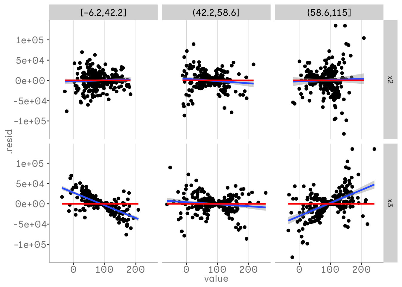

This becomes clearer when we plot x3, as our bins and both x1 and x2 still vary.

m3 %>%
  broom::augment() %>%
  mutate(x3 = dvmisc::quant_groups(x3, 3)) %>%
  pivot_longer(c(x1, x2)) %>%
  ggplot(aes(x = value, y = .resid))+
  geom_point()+
  geom_smooth(aes(x = value, y = .resid), method = "lm")+
  geom_smooth(aes(x = value, y = 0), col = "red", method = "lm")+
  facet_grid(vars(name), vars(x3))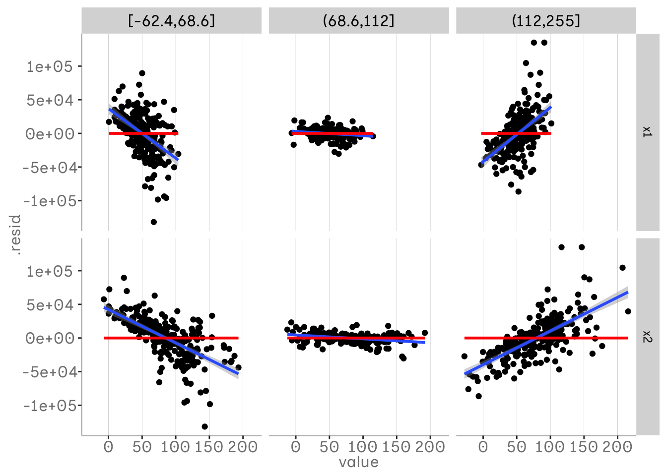

If you are working with real data, it may be helpful to use fewer bins and plot two of your three variables binned into quantiles.

m3 %>%
  broom::augment() %>%
  mutate(x3 = dvmisc::quant_groups(x3, 2)) %>%
  mutate(x2 = dvmisc::quant_groups(x2, 2)) %>%
  ggplot(aes(x = x1, y = .resid))+
  geom_point()+
  geom_smooth(aes(x = x1, y = .resid), method = "lm")+
  geom_smooth(aes(x = x1, y = 0), col = "red", method = "lm")+
  facet_grid(vars(x2), vars(x3))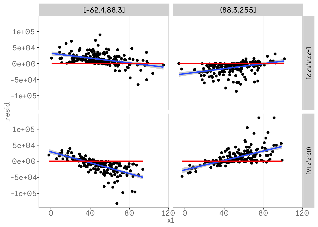

Whilst our residuals are currently centred on our model predictions, we can also plot the model adding back the fitted values from the augment ouput to the residuals. This allows us to plot our predicted slopes for the two way interaction and thus the effects of the third variables on those slopes. In other words, we can interpret how our two-way interaction varies with our third variable, e.g. x1 and x2 vary with x3.

m3 %>%
  broom::augment() %>%
  mutate(.resid = .fitted + .resid) %>%
  mutate(x3 = dvmisc::quant_groups(x3, 2)) %>%
  mutate(x2 = dvmisc::quant_groups(x2, 2)) %>%
  ggplot(aes(x = x1, y = .resid))+
  geom_point()+
  geom_smooth(aes(x = x1, y = .resid), method = "lm")+
  geom_smooth(aes(x = x1, y = .fitted), col = "red", method = "lm")+
  facet_grid(vars(x2), vars(x3))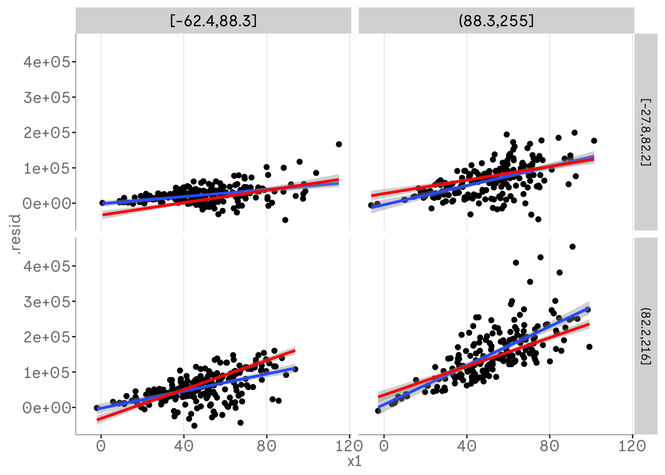

Beyond reverse engineering

In all of our plots so far, we have shown the residuals of our model against a variable that is already an independent variable in the model. However, we do not need to do this. This allows us to plot a variable against our response variable while controlling for another variable.

For example, we might be interested in including x1 in the model. So we just want to plot x1 against y while controlling for x2. Compared to plots with added variables, subtracting the predictor variable and fitting a visual regression to these residuals is not just an approximation of the regression slope, but rather an accurate estimate. Using the same methods as above, e.g. binning the other variable x2, we can also detect interactions before even fitting x1 into the model.

m4 <- lm(y_av ~ x1 + x2 + x3)

m4 %>%
  broom::augment() %>% 
  mutate(.resid = .resid + m0$coef[["x1"]] * x1) %>%
  mutate(x2 = dvmisc::quant_groups(x2, 3)) %>%
  ggplot(aes(x = x1, y = .resid))+
  geom_point()+
  geom_smooth(method = "lm")+
  facet_wrap(vars(x2))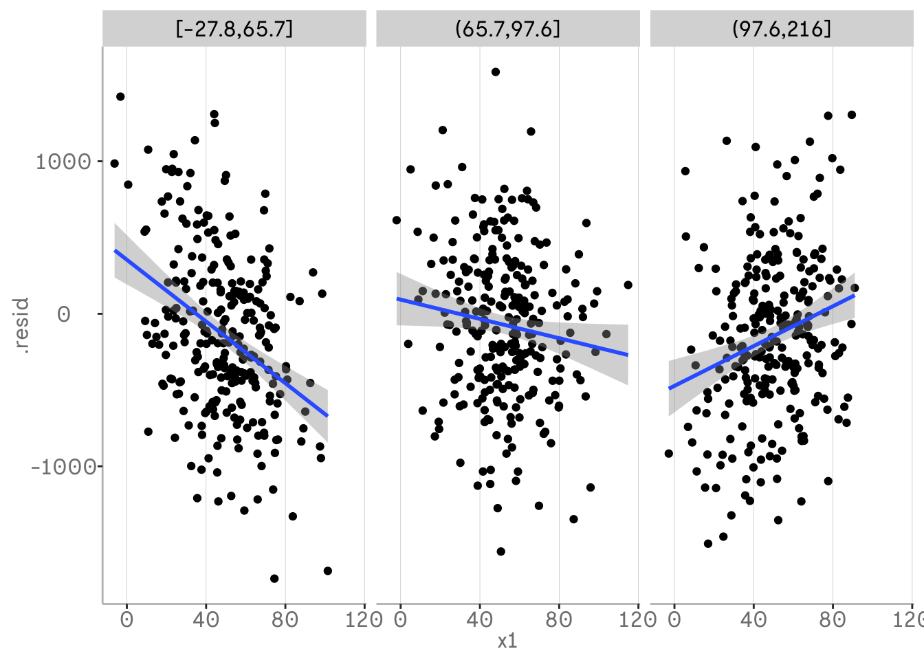

Additional notes

That was a lot of scatterplotting. Remember that it can be helpful to scale and centre your variables for plotting.

Literature

Fife, D. (2021). Visual Partitioning for Multivariate Models: An approach for identifying and visualizing complex multivariate dataset. https://doi.org/10.31234/osf.io/avu2n